Machine Learning

After having measured and extracted the acoustic variables, they are used to classify sounds – respectively feature values – in speech segments. The tools employed in the VokalJäger originate from the field of machine learning.

THE FLOATING PHONETIC FEATURE

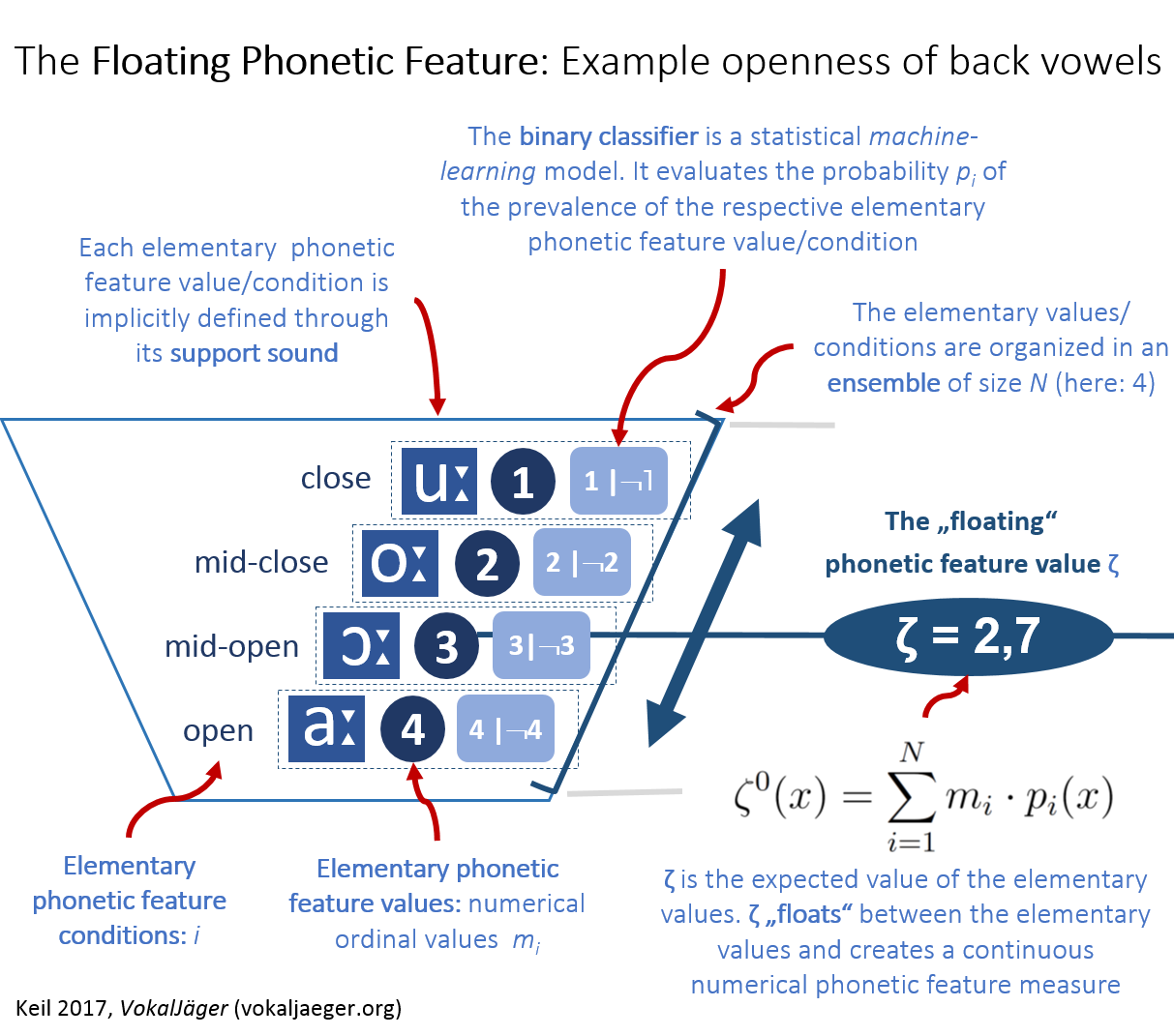
Classical phonetics assumes ordinal – that is: step wise – feature values, which often are binary. A particular front vowel is e.g. either round, like German [y:], or not-round, like its German counterpart [i:]. The values – in the setting used in the VokalJäger – don’t necessarily have to be binary: the openness of back vowels could be represented in the numerical value series 4, 3, 2 and 1, which represent open, mid open, mid close and close.

The situation becomes a bit tricky when small variations around those elementary values should be described. Classical phonetics employs the use of diacritics.

THE FLOATING PHONETIC FEATURE AND ITS VALUE

In the VokalJäger a different concept is utilized. It is assumed that, given a speech segment, a probability p can be evaluated to indicate how likely it is that, say, the vowel indeed is open, mid open, mid close or close. If one uses an ensemble of N numerical elementary phonetic feature values, e.g. m = 4, 3, 2 and 1, it is possible to mathematically evaluate an expected value. The elementary phonetic feature values constitute an ordinal representation of the underlying elementary phonetic feature conditions, here: open, mid open, mid close and close. This expected value, mathematically, shall be called floating phonetic feature value and be denoted by the Greek letter zeta ζ [Keil 2017, formula (35), p. 171; note the superscript 0: this particular ζ constitutes the initial floating phonetic feature value, from which, by means of order statistics, the final version is derived]. The key idea of the floating phonetic feature value is that ζ “floats” between the classical ordinal feature values (here: elementary phonetic feature values m): diacritics are now replaced by small numerical variations around the elementary values m. As result, a floating phonetic feature was constructed with an associated numerical value ζ.

SUPPORT AND CONTRAST SOUNDS

The probabilities p are calculated in a particular way: it is assumed, that for each elementary phonetic feature condition i – and hence: its associated elementary phonetic feature values m – certain sounds can be selected as representative – the so called support sounds. One may, e.g. have the elementary phonetic feature condition mid open for back vowels be represented by the support sound [ɔ] and assign the elementary phonetic feature value m = 3. Correspondingly there are so called contrast sounds – those being the sounds, which do not possess the respective elementary phonetic feature condition. The vowels [o:] and [a:] may e.g. be chosen as contrast sounds for the elementary phonetic feature condition mid open, respectively m = 3. Hence [o:] and [a:] form a representation for those sounds not showing the condition mid open, those not being m = 3, i.e. those with m ≠ 3.

BINARY CLASSIFIERS

In practice the probabilities are calculated using mathematical models. Employing machine-learning techniques, it is possible to train so called binary classifiers to detect existence respectively non-existence of singular elementary phonetic feature conditions (respectively: detect the prevalence of support sounds).

CONTRAST GROUPS AND PHONETIC FEATURE DIFFERENCES

Once the floating phonetic feature values ζ have been evaluated for certain groups, the next question is: do those ζ significantly differ between two groups? That can be answered by looking at the numerical differences statistically. Firstly the ζ center – mathematically: the median – of each group is evaluated (more precise: the center of the centers within same words):

[Keil 2017, formula (36), p. 183]. Then the numerical absolute difference is calculated and the statistical significance of the difference is considered:

[Keil 2017, formula (37), p. 187]. This measure – the phonetic feature distance Δζ – constitutes a probability weighted phonetic difference. To qualify as “significant” in above formula, the differences of the medians have to be statistically significant at least on the 95% level and the numerical absolute difference must exceed 0.25, what “equates” about to “half” a diacritic.

If one assembles the groups based on items, which are phonetically / phonologically distinct, those groups should contrast each other’s when looking at the floating phonetic feature values ζ – i.e. they should show significant feature distances Δζ. Groups which are hypothesized to differ are labelled VokalJäger’s contrast groups.

EXAMPLE: DIFFERENCES IN HIGH GERMAN O SOUNDS

The following picture exemplifies the concept of the phonetic feature distance Δζ on the scale of the floating phonetic feature of openness of back vowels. High German sounds from the Kiel PHONDAT Corpus were assembled into two contrast groups, one for the short O sounds, in High German mid open [ɔ], and a second for long O sounds, in High German mid closed [o:].

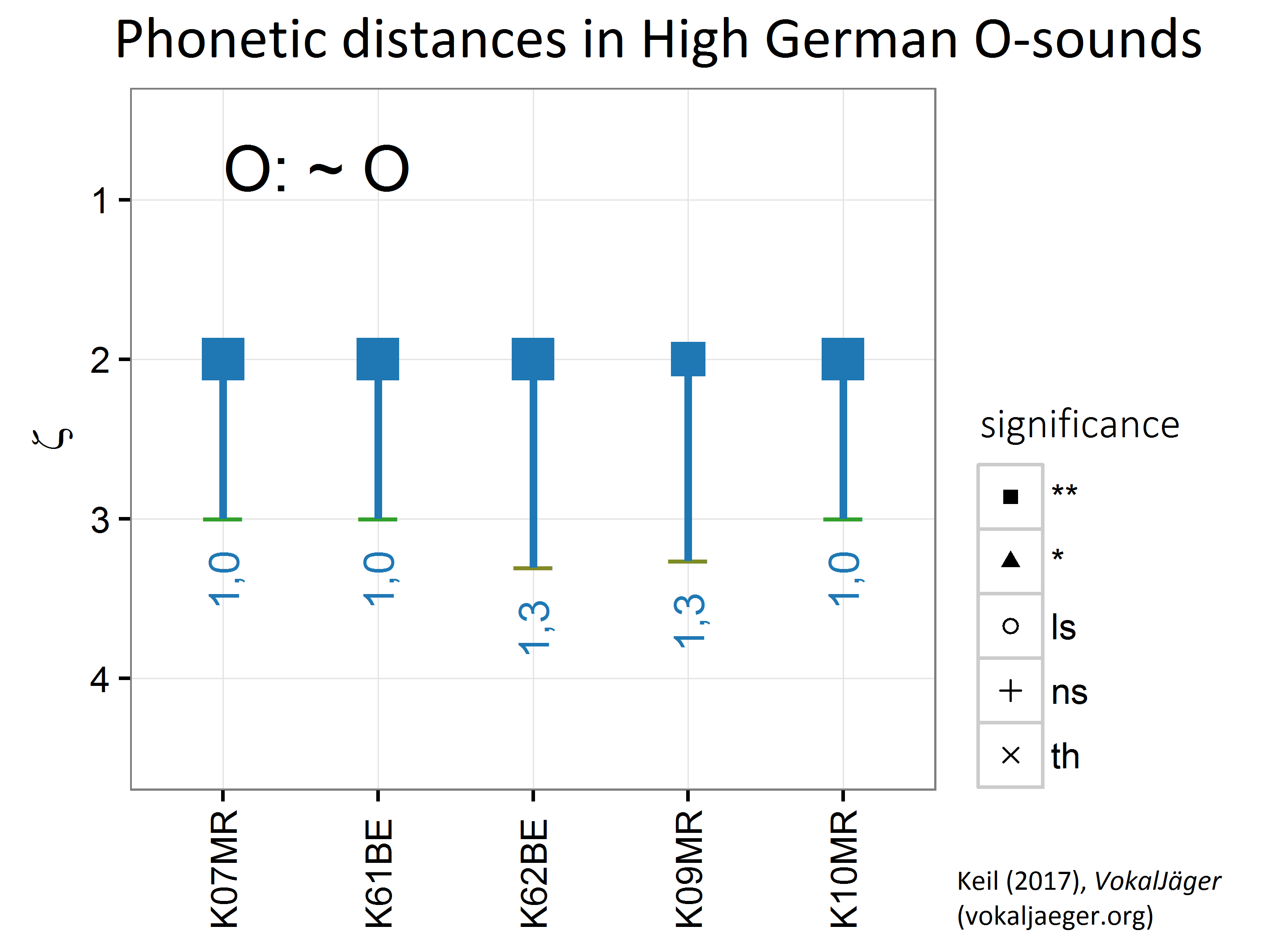
It can clearly be observed that High German short O-s assemble around ζ values of 3 – as expected for [ɔ]. The long O-s land contrarily at ζ values of 2 – as expected for [o:]. In all cases there are distances, which are are highly significant at the 99% level. The between-group distances range from Δζ = 1.0 to Δζ = 1.3 in this example.

Here one re-confirms with the VokalJäger text book knowledge: German short and long O sounds are qualitatively separate sounds.

BINARY CLASSIFIERS

Using machine learning, more precisely Kuhn (2015)’s wrapper CARET for numerous machine-learning algorithms in R, it is possible to build so called binary classifiers. The binary classifiers form the backbone of the VokalJäger‘s classification engine and are trained to detect the prevalence of certain elementary phonetic conditions.

The statistical Gaussian Mixture Discriminant Analysis (MDA) model was found to perform well in the VokalJäger vowel feature classification task [Hastie/Tibshirani 1996; Leisch/Hornik/Ripley 2013; full description in Keil 2017, p. 170–224]. Other models have been tested as well: Support Vector Machines, Neural Networks, Random Forests and K-Nearest Neighbours (KNN) yielded decent results at the level of the MDA, while more simpler ones like the Linear Discriminant Analysis (LDA) fell behind. Binary Classifiers trained with repeated cross validation on the first three formant values (which have been robustly Lobanov-normalized) yielded the most promising and most robust set up. In its default setting the VokalJäger classifies German vowels using mixture discriminant analysis and the formants F1 to F3.

THE RESPONSE OF THE BINARY CLASSIFIER

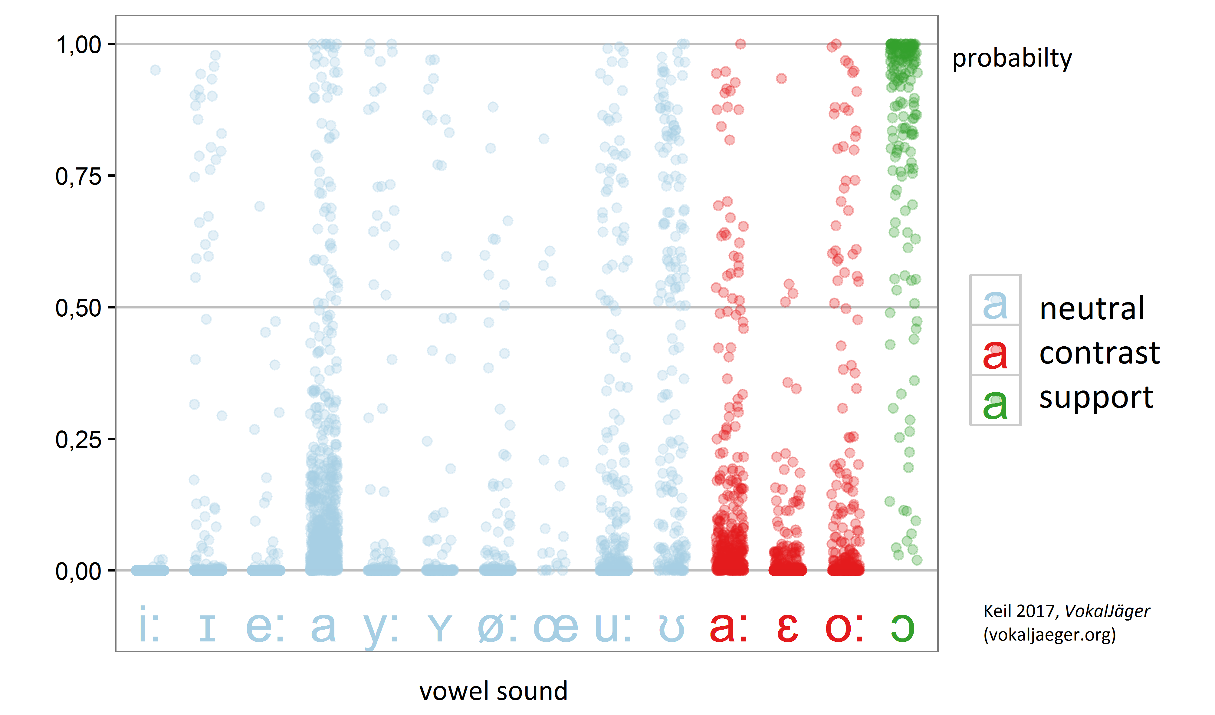
Below exemplary chart shows the response of a VokalJäger MDA binary classifier (here: based on the F1/F2 formants only), which was trained to detect the vowel [ɔ]. In the setting of the floating phonetic feature openness of back vowels the [ɔ] constitutes the support sound of the elementary phonetic feature value m = 3, this is: mid open. The plotted response on the scale 0 to 1 is a measure of the probability p that the speech sound indeed occurs to be an [ɔ]. As can be seen, the binary classifier performs as expected: the support sounds [ɔ] are usually detected (responses > 0.5), while most of the contrast sounds [a:/ε:/o:] are rejected by the binary classifier (responses < 0.5). The neutral sounds, which are omitted from the training, perform by phonetic proximity: e.g. [a] is rejected as is the contrast sound [a:].

BINARY CLASSIFIERS: RESULTS IN THE F1/F2 PLANE

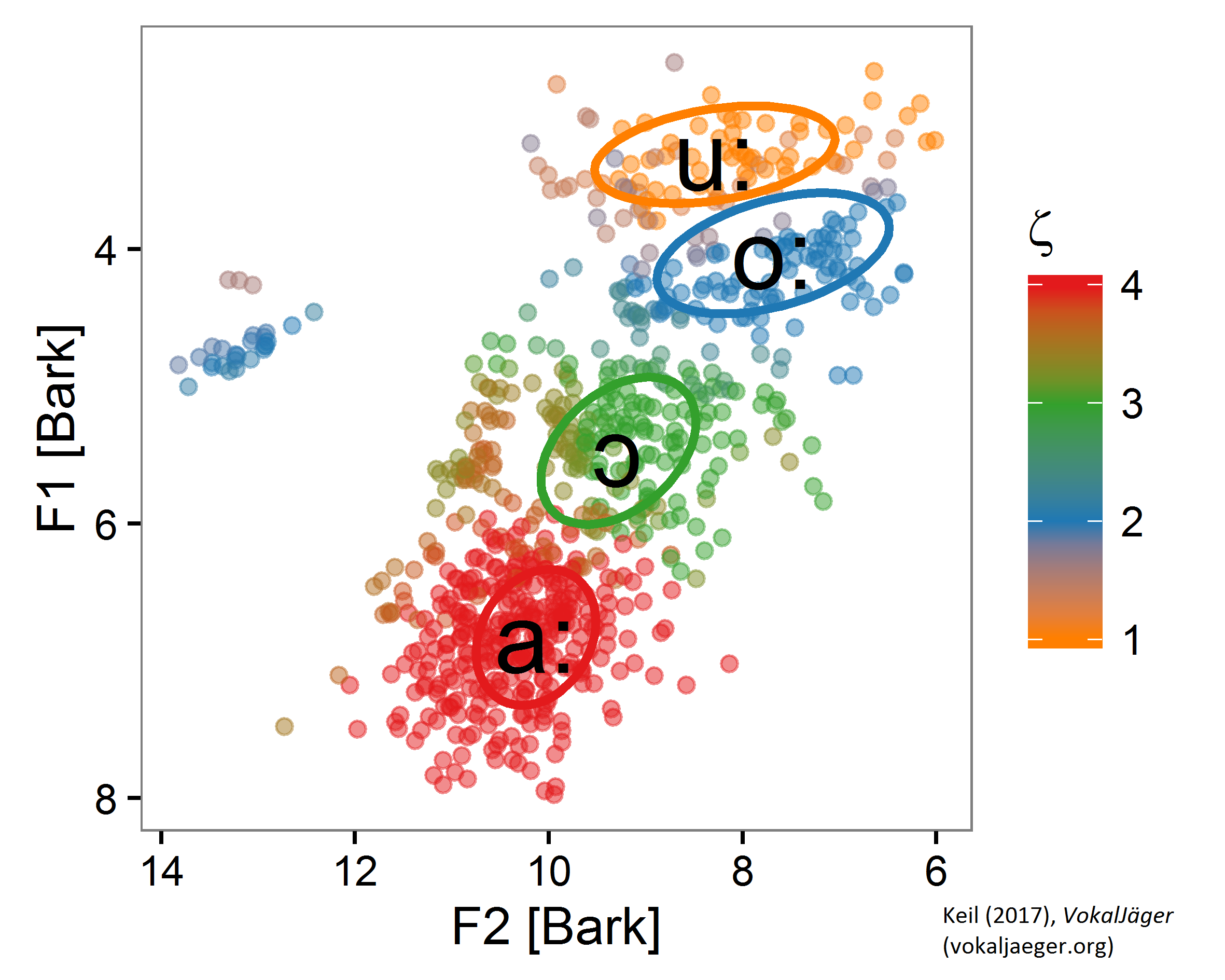
If one assembles different binary classifiers together in an ensemble, one recognizes them detecting the “correct” sounds – respectively throwing a positive answer when fed with acoustic variables originating from the respective “area” in the F1/F2-plane. That is shown in below picture, which shows by color which binary classifier “wins” in the ensemble and indicates what sound was found. The colors nicely align with “areas” the corresponding vowels usually “occupy”, what is indicated with the ellipses.

BINARY CLASSIFIERS: HERE I AM

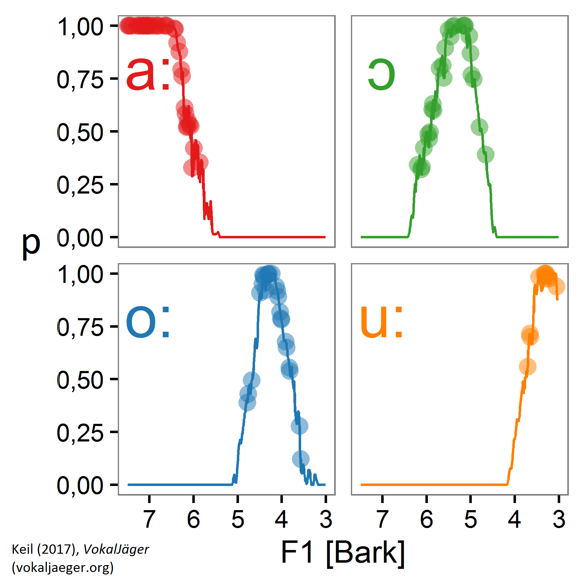
If one “walks” a “line” through the F1/F2-plane, touching (in order) the [a:], [ɔ], [o:] and [u:] “areas”, the individual binary classifiers throw probabilities to indicate the supposed prevalence of the sound they have been trained on – comparable with a cry “here I am”. As measure for the location in the F1/F2 plane here F1 is plotted as x-axis, basically the vertical position in an F1/F2 chart. One can clearly recognize the binary classifiers knocking in and fading out:

ASSEMBLING BINARY CLASSIFIERS INTO FLOATING PHONETIC FEATURES

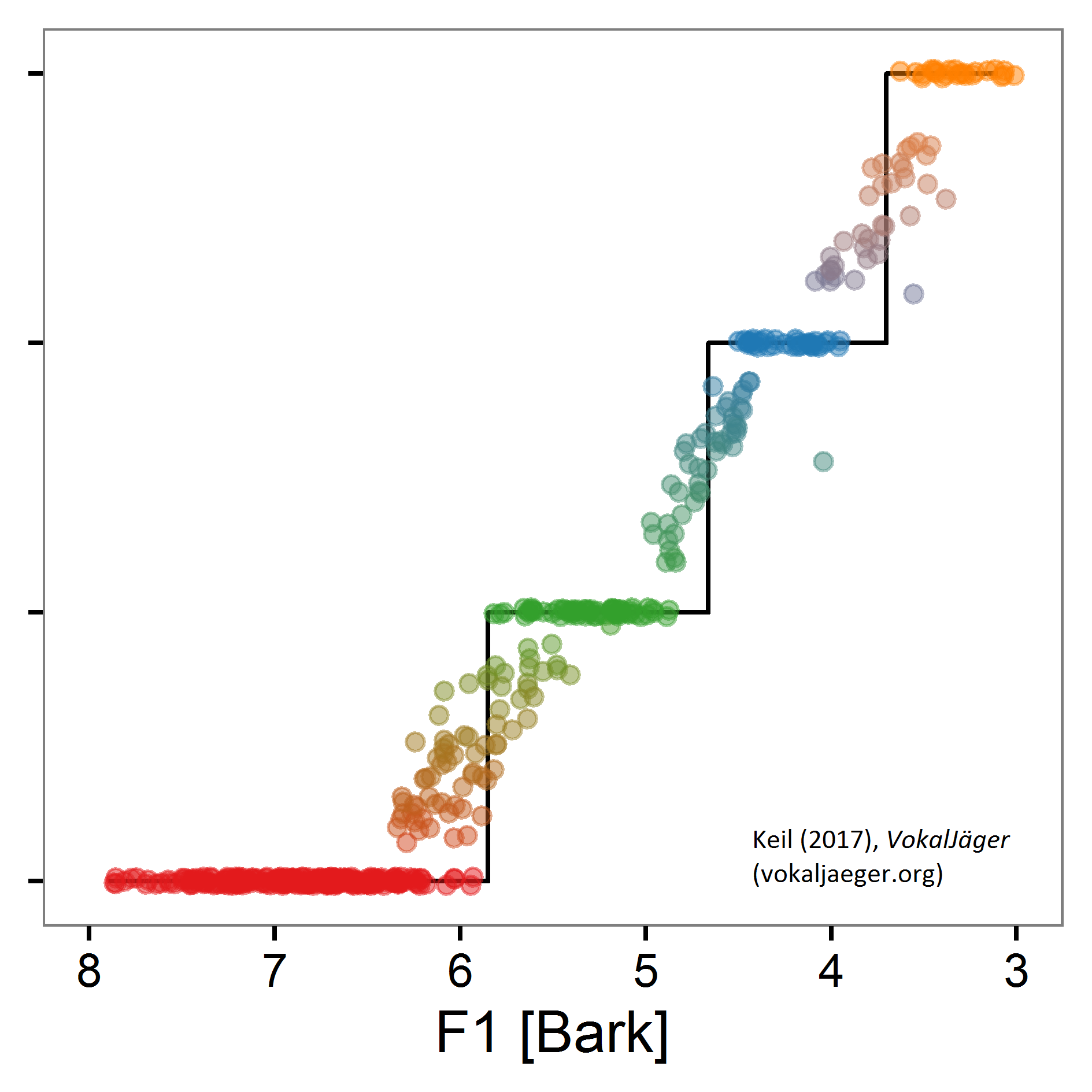
From the individual binary classifiers’ probability values it is now possible to calculate the floating feature value ζ, what is shown in the next diagram. One can observe the desired pattern: When walking the line between the [a:], [ɔ], [o:] and [u:] “areas”, the floating feature value ζ “jumps” between the elementary feature values m = 4, 3, 2 and 1. There is some clustering, literally forming a “staircase” – those being the values associated 1:1 with the winning binary classifier. On the other side there is some intermediate migration in between – those being the values usually described with diacritics.